Skewness

Skewness:

In Statistics we have numerous distribution and every distribution has his own graph and interpretation. Likewise, in skewness we use central tendency (Mean, Mode, Median) and construe it accordingly. Therefore, skewness is a tool that assist us to interpret  central distribution or central location through  following three ways:

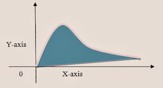
Positively Skewed:

In positively skewed, mean is always greater as compare to mode, median and mode is always less then median. In mathematically we can write it as:

Mean > Median> Mode = Mode< Median< Mean

Here graph shows that the data is Positively skewed and has right tail.

Negatively Skewed:

In negatively skewed, mode is always greater as compare to mean and median, mean is always less then median. In mathematically we can write it as:

Mean < Median < Mode = Mode >Median > Mean

Here graph shows that the data is Natively skewed  and has left tail.

Symmetric  or Skewed:

In symmetric or skewed, mean, mode and median are equal to each other and it has no tail.

Mean = Mode=Median

Here graph shows that the data is symmetric.

Measures of dispersion

Measures of Dispersion
Introduction:

Measures of dispersion are descriptive information that explains how connected set of scores are comparable to each other. Statistician know the  dispersion as  variability, scatter, or spread. Dispersion is contrasted with location or central tendency, and together they are the most used properties of distributions. Using dispersion, a person can easily interpret how stretched or squeezed is a distribution . The most common measures of statistical dispersion are the variance, standard deviation and interquartile range.

 

A measure of statistical dispersion is a nonnegative real number that is zero if all the data are the same and increases as the data become more diverse. Most measures of dispersion have the same units as the quantity being measured. In other words, if the measurements are in meters or seconds, so is the measure of dispersion. Dispersion  is very sensitive to outliers and does not use all the observations in a data set. It is more informative to provide the minimum and the maximum values rather than providing the range.

 

Standard Deviation:

Standard deviation (SD) is the most commonly used measure of dispersion. It is a measure of spread of data about the mean and it is the square root of sum of squared deviation from the mean divided by the number of observations. In Statistics we have two formulas to calculate SD.

1. For sample SD:

In sample SD formulas we use n - 1 instead of n in the denominator, because this produces a more accurate estimate of sample SD.

2. For population SD:

 

 

  Range:

This spread measure, which is sometimes used , is defined as the difference between the highest and lowest values.

 

 

Interquartile range:

This measure is defined as the difference between the 1st and 3rd quartiles.

 

Variance:

Variance is defined as the measure obtained by adding together the squares of the deviation of the sample values from their mean, and dividing the result by the number of values in sample.

We calculate the Variance as:

1.For Sample Variance:

2. For Population Variance: 

 

 

 

 

Measures of Central Tendency

Measures of Central Tendency

Introduction:

A measure of central tendency is a single value that attempts to describe a set of data by identifying the middle or the center  position within that set of statistics. It is occasionally called an average, center of the distribution,  measures of central location and  also classed as summary statistics. The mean often called the average is most likely the measure of central tendency that you are most familiar with, but there are others, such as the median and the mode. The mean, median and mode are all valid measures of central tendency, but under different conditions, some measures of central tendency become more appropriate to use than others.

Mean:

Mean is what most people commonly refer to as an average. It can be used with both discrete and continuous data, although its use is most often with continuous data. The mean is equal to the  sum up a given set of numbers and then divide this sum by the total number in the set. Mean is also referred to more correctly as arithmetic mean. In statistics there are two kinds of means: population mean and sample mean. A population mean is the true mean of the entire population of the data set while a sample mean is the mean of a small sample of the population. So, if we have n values in a data set and they have values x₁, x₂, ..., x_n, the sample mean, and it is pronounce by X bar:

 

This formula is usually written in a slightly different manner using the Greek capitol letter,∑, pronounced "sigma", which means "sum":

Population mean is represented by the Greek letter μ pronounced mu. The total number of elements in a population is represented by N:

The sample mean is commonly used to estimate the population mean when the population mean is unknown. This is because they have the same expected value.

Median:

The median is defined as the number in the middle of a given set of numbers arranged in order of increasing magnitude. When given a set of numbers, the median is the number positioned in the exact middle of the list when you arrange the numbers from the lowest to the highest. The median is important because it describes the behaviour of the entire set of numbers. For example, we have a set of number

15, 16, 15, 7, 21, 18, 19, 20, 11

From the definition of median, first step is to rearrange the given set of numbers in order of increasing magnitude:

7, 11, 15, 15, 16, 18, 19, 20, 21

Then we inspect the set to find that number which lies in the exact middle.

Median = 16

So, if we look at the another example that often occurs when solving for the median.:

65

55

89

56

35

14

56

55

87

45

We again rearrange that data into order of magnitude (smallest first):

14

35

45

55

55

56

56

65

87

89

92

Only now we have to take the 5th and 6th score in our data set and average them to get a median of 55.5.

Mode:

The mode is defined as the element that appears most frequently in a given set of elements. On a histogram it represents the highest bar in a bar chart or histogram. Therefore, sometimes consider the mode as being the most popular option.

For example, in the 3, 3, 6, 9, 16, 16, 16, 27, 27, 37, 48 are the set of numbers,  here 16 is the mode since it appears more times than any other number in the set.
A set of numbers can have more than one mode this is known as bimodal, if there are multiple numbers that occur with equal frequency, and more times than the others in the set.
3, 3, 3, 9, 16, 16, 16, 27, 37, 48
In this example, both the number 3 and the number 16 are modes.
If no number in a set of numbers occurs more than once, that set has no mode:
3, 6, 9, 16, 27, 37, 48
in this list there is no mode.

Foundation of Statistics

Foundation of Statistics

Statistics is fundamentally concerned with the presentation and interpretation of chance outcomes that occur in a planned or scientific investigation. Many Statistician, Theorist and Scientist came in different ages; they define the Statistics differently. Some consider statistics as mathematical body of science that pertains to the collection, analysis, interpretation or explanation, and presentation of data while others consider it a branch of mathematics concerned with collecting and interpreting data. Because of its experimental roots and its focus on applications, statistics is usually considered a distinct mathematical science rather than a branch of mathematics. Some tasks a statistician may involve are less mathematical; for example, ensuring that data collection is undertaken in a way that produces valid conclusions, coding data, or reporting results in ways comprehensible to those who must use them. Statisticians improve data quality by developing specific experiment designs and survey samples. Statistics itself also provides tools for prediction and forecasting the use of data and statistical models. Statistics is applicable to a wide variety of academic disciplines, including natural and socialsciences, government, and business. Statistical consultants can help organizations and companies that don't have in-house expertise relevant to their particular questions. For example, a Statistician wants to record the number of accidents that manly occur from the interaction of E.walnut str and S.Galbstone ave in Jordan valley park, Springfield. The Statistician hoping to justify the installation of traffic lights, he might classify responses in an opinion poll " Yes" or "No". Therefore, the Statistician is usually dealing his data either  numerical data or Qualitative data.

In daily life, a person work on different applications and these all have their own progression to have done them. Therefore, working on statistics, it’s important to recognize the different types of data. Data are the actual pieces of information that a person collect through his studies. For example, if a person asks six of his friends how many pets they own, they might give him the following data: 0, 6, 2, 1, 4, 18. Not all data are numbers; let’s say a teacher  also record the gender of each of his students, getting the following data: male, male, female, male, female. Most data fall into one of two groups: numerical or Qualitative.

 ·   Numerical data: Statisticians also call numerical data as quantitative data. These data have meaning as a measurement, such as a person’s height, weight, IQ, or blood pressure; or they’re a count, such as the number of stock shares a person owns, how many teeth a dog has, or how many pages you can read of your favourite book before you fall asleep. Numerical data is further broken into two types: discrete and continuous.

o  Discrete data it take on possible values that can be listed out. For example, the number of heads in 100 coin flips takes on values from 0 through 100 finite case, but the number of flips needed to get 100 heads takes on values from 100 the fastest scenario on up to infinity. If you never get to that 100th heads, it's possible values are listed as 100, 101, 102, 103, . . . representing the countably infinite case.

o Continuous data represent measurements; their possible values cannot be counted and can only be described using intervals on the real number line. For example, the exact amount of gas purchased at the pump for cars with 20-gallon example tanks would be continuous data from 0 gallons to 20 gallons, represented by the interval [0, 20], inclusive. You might pump 8.40 gallons, or 8.41, or 8.414863 gallons, or any possible number from 0 to 20. In this way, continuous data can be thought of as being unaccountably infinite.

· Qualitative data: When things are grouped accordingly some common property and the number of members of the group are recorded e.g. males/female, vehicle types.

In Statistics there are two statistical methods to collection, presentation, analysis and interpretation of data.

Descriptive Statistics consist of those methods concerned with collection and describing a set of data so as to yield meaningful information. For example, construction of tables, charts, graphs, and other relevant computation in various newspapers and magazine usually fall in the area categorized as descriptive statistics. In the other hand, Statistical Inference comprise those methods concerned with the analysis of a subset of data leading to prediction or inference about the entire set of data.